Appendix E: Block-Circulant CHM
created: 2026-09-13
updated: 2026-09-20 by W. Bruzda
Not every file in the repository is listed on this page. The collection grows faster than these tables – for the complete set, browse the repository directly.
The matrices collected here come from "Block-Circulant Complex Hadamard Matrices" [175]. They are numerical, not analytic and each one is a solution of the unitarity constraints imposed on a block-circulant pattern, found with fsolve and refined until the residual reaches machine precision.
Two sequences are solved here:
The two sequences are structurally different, which is easy to miss because they are solved the same way. LN is bordered group-developed meaning its core is H(g, h) = F(h - g) over the cyclic group of order N - 1, written Zn × Z2 with n = (N - 1)/2 odd and with F(m, 1) = conj(F(m, 0)). Hence, it is a circulant-core matrix in the sense of Nicoară and Worley [182], although their finiteness theorem concerns a core of prime size and the core here has order N - 1 = 2n with n odd, composite for every N ⩾ 7. The group is recovered from every LN here by CHM_GH/gh_check.py. Appendix F sweeps the same construction over arbitrary groups and these matrices came first and are not listed there. VN is not of that form as it starts from an unbordered circulant matrix of order N and 83 of its 85 matrices of order at most 40 fail a necessary condition for group development that does not depend on how the group is labelled. The two that do not fail are V7,0,7 and V11,0,11, the entries marked below as F7 and F11 in disguise and for those a bordered group-developed representative does exist. The matrices below are not duplicated in Appendix F and the ones its sweep rediscovered (for N = 11, 15, 19) are recorded there as already catalogued and the classes it lists over the same cyclic groups at N = 23 and 27 were checked to be monomially inequivalent to these.
Their interest is that almost every solution turns out to be isolated (defect d = 0) and not of Butson type. For LN one obtains isolated solutions only while for VN other defects occur as well. Since the sequences can be run in essentially any dimension, they provide numerical support for the conjecture that isolated complex Hadamard matrices exist in every dimension – a question left open by the analytic constructions, which supply isolated examples only in special dimensions (Fourier Fp for prime p, S6 and not many others).
For the initial dimensions 11–16 each run returns different values of the parameters and whether the resulting matrices are inequivalent is not known.
filename scheme↑
Every file stores the phase matrix A, so that H = exp(2πi·A) is the complex Hadamard matrix itself:
LH_N_d_L.data   block-circulant, sequence L
VH_N_d_L.data   block-circulant, sequence V

        N = size(H)
        d = defect(H)
        L = #Λ(H), cardinality of the Haagerup set
Both invariants are expensive, so they are recorded only while that is affordable and the name degrades in a fixed way:
N ⩽  40      LH_N_d_L.data     both invariants
N ⩽  60      LH_N_d.data       #Λ too slow to compute
N >  60      LH_N.data         both too slow to compute
A trailing letter distinguishes different solutions that share the same invariants (VH_14_0_687A, ...B, ...) and a trailing word records a property worth keeping (_persymmetric, _BH).
scripts↑
The two generators write a ready-to-run Octave M-file for a given dimension. Running it solves the system and saves the solution under the name above.
$ ./BC_L.sh 11          # writes LH_11.m
$ ./C_V.sh 10           # writes VH_10.m

octave:1> H = LH_11;    # solves, then saves LH_11_0_191.data
bc_name.m builds the file name and is the only helper the generated M-files need. It also calls ud.m for the defect.
LN works only for N = 3 + 4k; the number of parameters is (N - 1)/2. For N > 55 the invariants take too long and the name is shortened automatically.
sequence LN↑
Solvable for N = 3 + 4k only. Every converged solution found so far is isolated.
Both invariants below are computed numerically, from a floating-point representation of H. The Haagerup set is obtained by forming all N4 products HijHklHilHkj and counting how many distinct values remain. The count recorded here is the one produced by bc_name.m, which rounds the real and imaginary parts onto a grid of step 10-6 and counts the occupied cells. That is a quantisation, not a test of distance so two values closer than the step are still counted twice when they fall either side of a cell boundary and two values further apart than the step can share a cell. It is also not the convention used by CHM_tool/lambda, which compares distances and defaults to 10-8. Re-measured with that tool, 16 of the 102 labelled matrices below come out differently at 10-6 and 19 at 10-8 – VH40 reads 15985 here and 16001 there. So the figures for #Λ are labels at a stated resolution, not exact invariants and they may not be compared with another appendix without re-measuring both sides the same way. They are least reliable for large N, where the set is large and its elements lie close together and for any matrix whose residual is not at machine precision – VH_9_0_89C and VH_9_0_89D are stored with a Gram residual near 10-9 rather than 10-15, so their finer counts in particular carry no weight. Read them as characteristics useful for telling these matrices apart, not as exact invariants. The defect, being the rank of a real matrix, is markedly more stable, but it rests on a singular-value threshold of the same kind.
| matrix | defect | #Λ | comment |
|---|---|---|---|
| LH3,0,3 | 0 | 3 | ≅ F3 ∈ BH(3, 3) |
| LH7,0,7 | 0 | 7 | ≅ F7 ∈ BH(7, 7) |
| LH11,0,191 | 0 | 191 | |
| LH11,0,191A | 0 | 191 | |
| LH11,0,191 | 0 | 191 | block persymmetric |
| LH15,0,463 | 0 | 463 | |
| LH15,0,463A | 0 | 463 | |
| LH15,0,463B | 0 | 463 | |
| LH19,0,919 | 0 | 919 | |
| LH23,0,1607 | 0 | 1607 | |
| LH27,0,2575 | 0 | 2575 | |
| LH27,0,2575A | 0 | 2575 | |
| LH31,0,3869 | 0 | 3869 | |
| LH31,0,3871 | 0 | 3871 | |
| LH35,0,5543 | 0 | 5543 | |
| LH35,0,5543A | 0 | 5543 | |
| LH39,0,7633 | 0 | 7633 | |
| LH39,0,7635 | 0 | 7635 | |
| LH43,0 | 0 | – | |
| LH43,0A | 0 | – | |
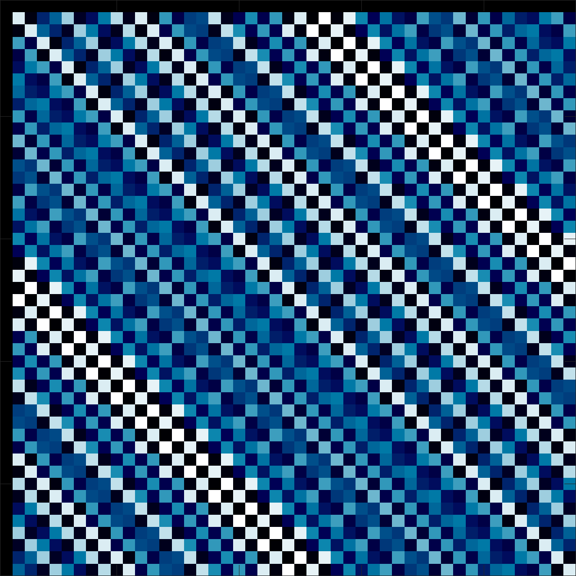
| LH47,0 | 0 | – | figure |
| LH47,0A | 0 | – | |
| LH51,0 | 0 | – | |
| LH55,0 | 0 | – | |
| LH59,0 | 0 | – | |
| LH63 | – | – | |
| LH67 | – | – | |
| LH71 | – | – | |
| LH75 | – | – | |
| LH79 | – | – | |
| LH83 | – | – | |
| LH87 | – | – | |
| LH95 | – | – | |
| LH99 | – | – | |
| LH103 | – | – | |
| LH107 | – | – | |
| LH111 | – | – | |
| LH115 | – | – | |
| LH123 | – | – |
sequence VN↑
Solvable in any dimension N ⩾ 6. Defects other than zero do occur.
Raw runs↑
Kept for the record, under their original names. These did not converge: either the residual is too large for the invariants to mean anything, or the result is not CHM at all. They are not part of the collection above.
| file | N | F-norm | comment |
|---|---|---|---|
circulant_L5.data | 5 | 1.5e+00 | not CHM |
circulant_V6.data | 6 | 6.7e-07 | unconverged (invariants unreliable) |
circulant_V6_1010.data | 6 | 1.1e+01 | not CHM |
circulant_V6_1020.data | 6 | 6.6e-01 | not CHM |
circulant_L9.data | 9 | 5.9e-01 | not CHM |
circulant_V9_40.data | 9 | 5.8e-07 | unconverged (invariants unreliable) |
circulant_V9_50.data | 9 | 8.1e-06 | unconverged (invariants unreliable) |
circulant_V9_60.data | 9 | 2.0e-06 | unconverged (invariants unreliable) |
circulant_V9_70.data | 9 | 2.2e-05 | unconverged (invariants unreliable) |
circulant_V9_80.data | 9 | 2.0e-05 | unconverged (invariants unreliable) |
circulant_V10.data | 10 | 5.0e-08 | unconverged (invariants unreliable) |
circulant_L23.data | 23 | 1.1e-07 | unconverged (invariants unreliable) |
circulant_V90.data | 90 | 2.3e+02 | not CHM |
circulant_L91.data | 91 | 8.7e+00 | not CHM |
circulant_L119.data | 119 | 8.6e+00 | not CHM |
circulant_L127.data | 127 | 1.9e+01 | not CHM |
circulant_V127.data | 127 | 3.4e+02 | not CHM |
The two random-walk files, rw_L11_1000.data and rw_L13_1000.data, hold a thousand-step walk around L11 and L13, not single matrices.